Drawing flowers using mathematics
For the love of arts, I’m going to make a flower in R.
Let’s start by drawing 50 points on a circle of radius 1. As every (x, y) point should be in the unit circle, it follows that x² + y² = 1. We can get this using the Pythagorean trigonometric identity which states that sin²(θ) + cos²(θ) = 1 for any real number θ.
It is important to know that in geom_point, the size of the circles are related to the coordinate system and not to a separate scale. So you don’t specify the radius. We will how to radius later.
library(tidyverse)

t <- seq(0, 2*pi, length.out = 50)
x <- sin(t)
y <- cos(t)
df <- tibble(t, x, y)

# Make a scatter plot of points in a circle
p <- ggplot(df, aes(x, y))
p + geom_point()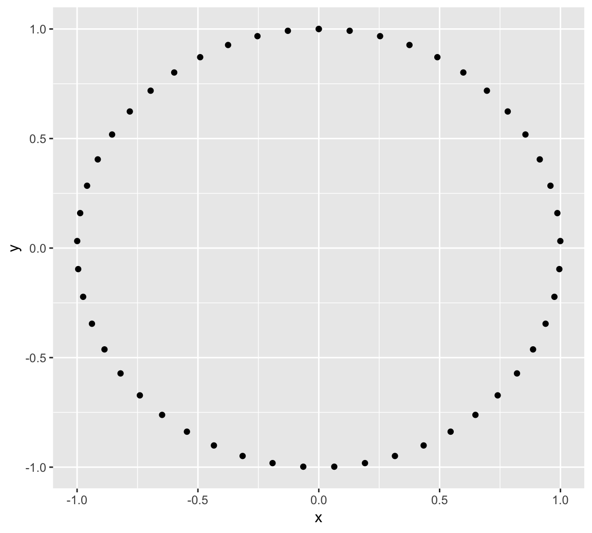
Golden Angle
The arrangement of leaves and many other things in nature is spiral. Check out this article on patterns in nature. A spiral starts from the origin and moves away from this point as it revolves around it. In the plot above all our points are at the same distance from the origin. A simple way to arrange them in a spiral is to multiply x and y by a factor which increases for each point. We could use t as that factor, as it meets these conditions, but we will do something more harmonious. We will use the Golden Angle:
Golden Angle = π(3 − √5)
This number is inspired by the Golden Ratio, one of the most famous numbers in the history of mathematics. Apart of flower petals and plant leaves, you’ll find them in seed heads, pine cones, sunflower seeds, shells, spiral galaxies, hurricanes, etc.
# Defining the number of points
points = 500

# Defining the Golden Angle
angle = pi * (3 - sqrt(5))

t <- (1:points) * angle
x <- sin(t)
y <- cos(t)
df <- data.frame(t, x, y)

# Make a scatter plot of points in a spiral
p <- ggplot(df, aes(x*t, y*t))
p + geom_point()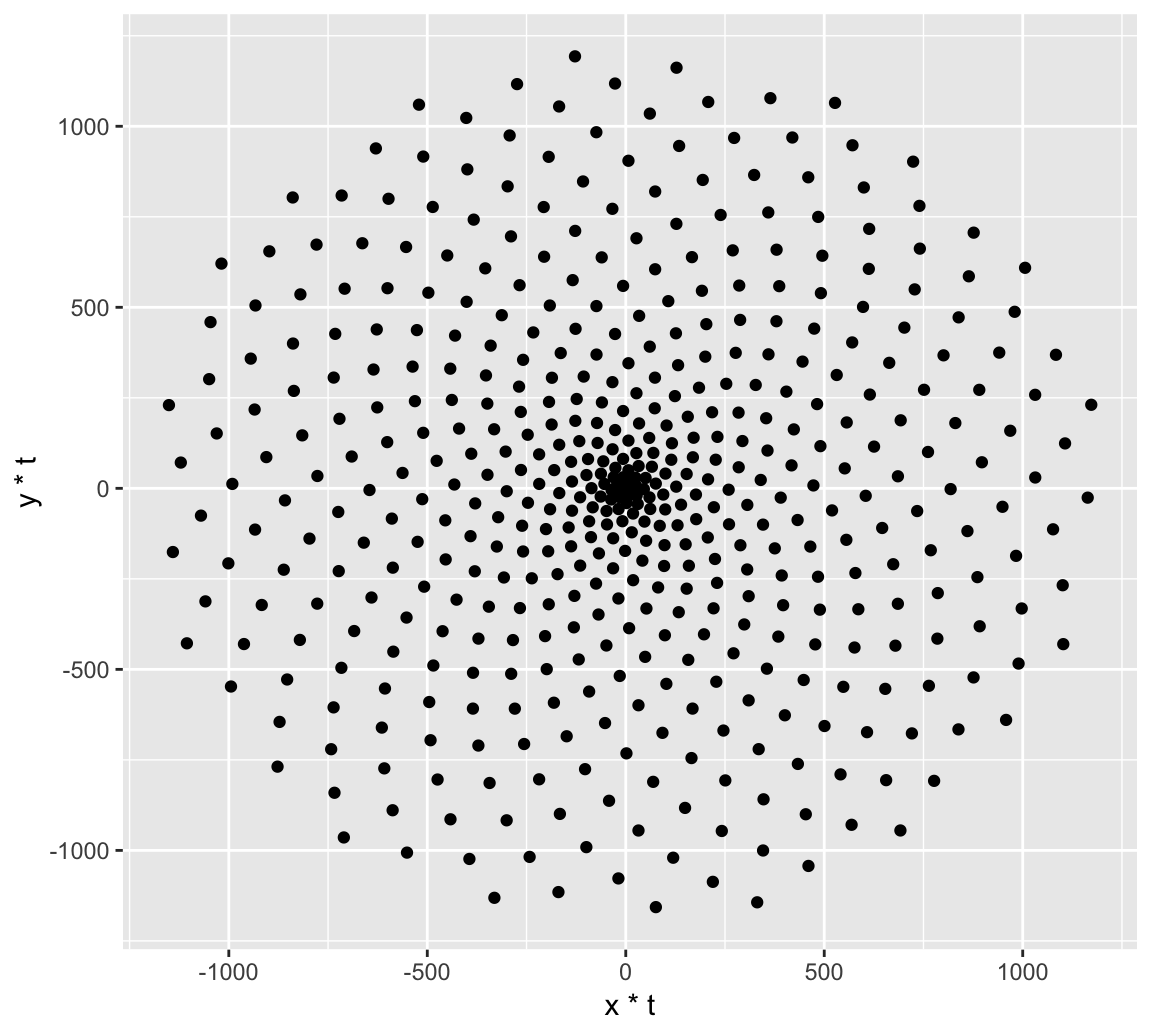
Let’s play around! Let’s try twice of the golden angle and increase the number of points by 10 times and see how things change!
# Defining the number of points
points_1 = 5000

# Defining the Golden Angle
angle_1 = 2*pi * (3 - sqrt(5))

t_1 <- (1:points_1) * angle_1
x_1 <- sin(t_1)
y_1 <- cos(t_1)
df_1 <- data.frame(t_1, x_1, y_1)

# Make a scatter plot of points in a spiral
p <- ggplot(df_1, aes(x_1*t_1, y_1*t_1))
p + geom_point()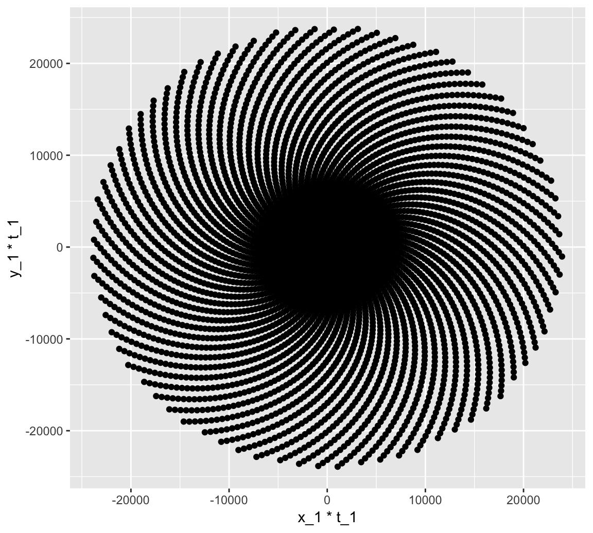
Time to clean up!
The code below sets the background color to white, and removes all elements of the x and y axes.
df <- data.frame(t, x, y)

# Make a scatter plot of points in a spiral
p <- ggplot(df, aes(x*t, y*t))
p + geom_point() + theme(legend.position = "none",
        panel.grid = element_blank(),
        axis.title = element_blank(),
        axis.text = element_blank(),
        axis.ticks = element_blank(),
        panel.background = element_rect(fill = 'white'))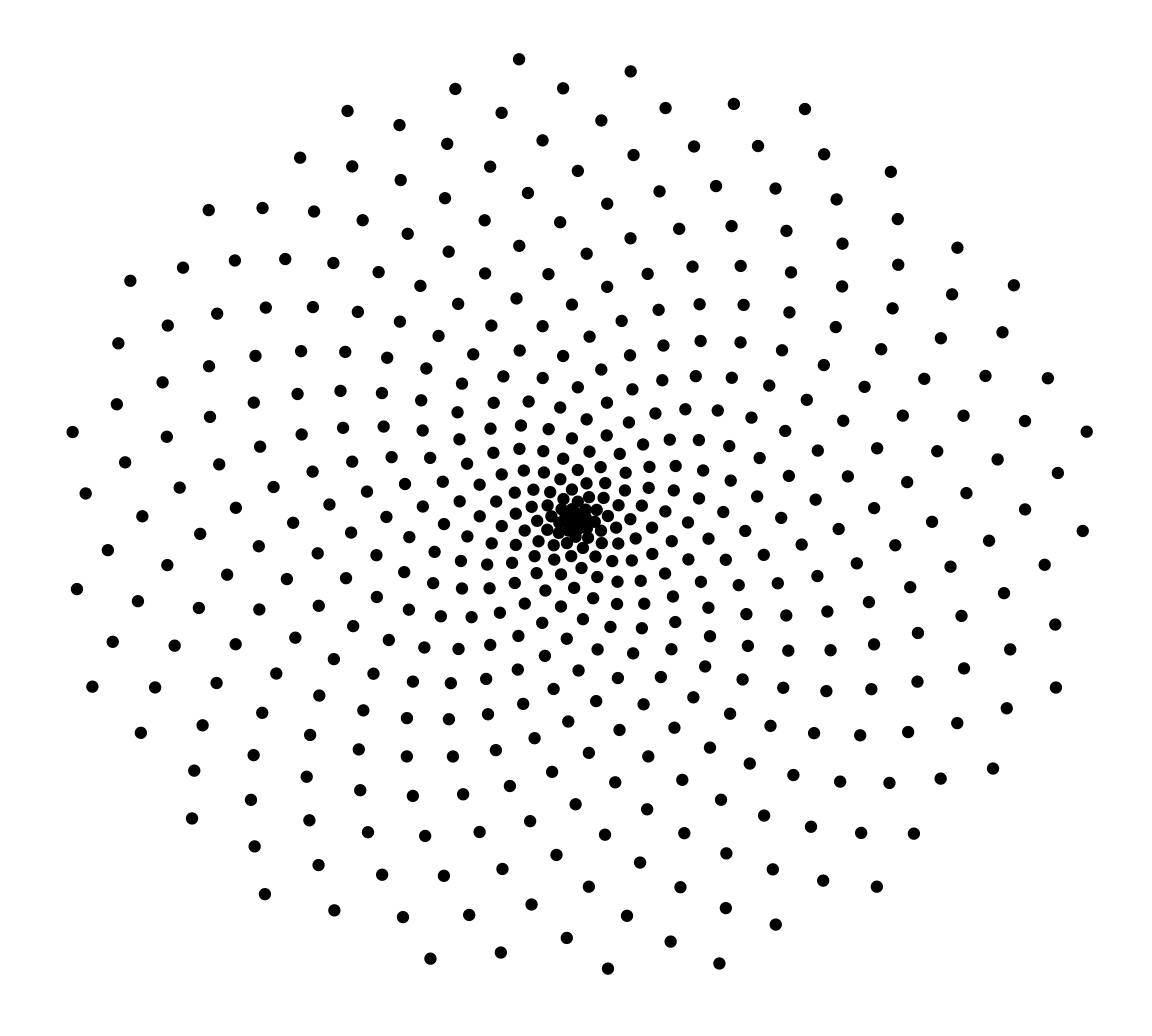
Coloring
Simply playing around the color schemes and shapes to get a good feel.
p <- ggplot(df, aes(x*t, y*t))
p + geom_point(size = 3, alpha = 0.5, shape = 22, fill = "darkcyan") + theme(legend.position = "none",
        panel.grid = element_blank(),
        axis.title = element_blank(),
        axis.text = element_blank(),
        axis.ticks = element_blank(),
        panel.background = element_rect(fill = 'white'))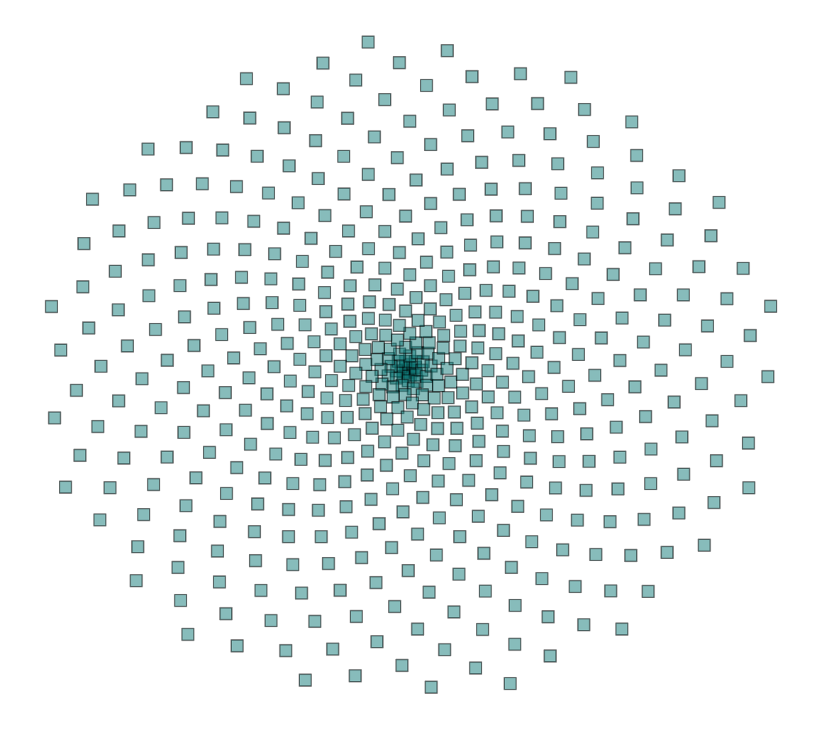
Angles
These patterns are very sensitive to the angle between the points that form the spiral; small changes to the angle can generate very different images
Let’s change the angle and increase the number of points from to 2000.
angle <-  pi/180
points <- 2000

t <- (1:points)*angle
x <- sin(t)
y <- cos(t)

df <- data.frame(t, x, y)

p <- ggplot(df, aes(x*t, y*t))

p + geom_point(size= 80, color = 'magenta4', alpha = 0.1, shape = 1) + theme(legend.position = "none",
        panel.grid = element_blank(),
        axis.title = element_blank(),
        axis.text = element_blank(),
        axis.ticks = element_blank(),
        panel.background = element_rect(fill = 'white'))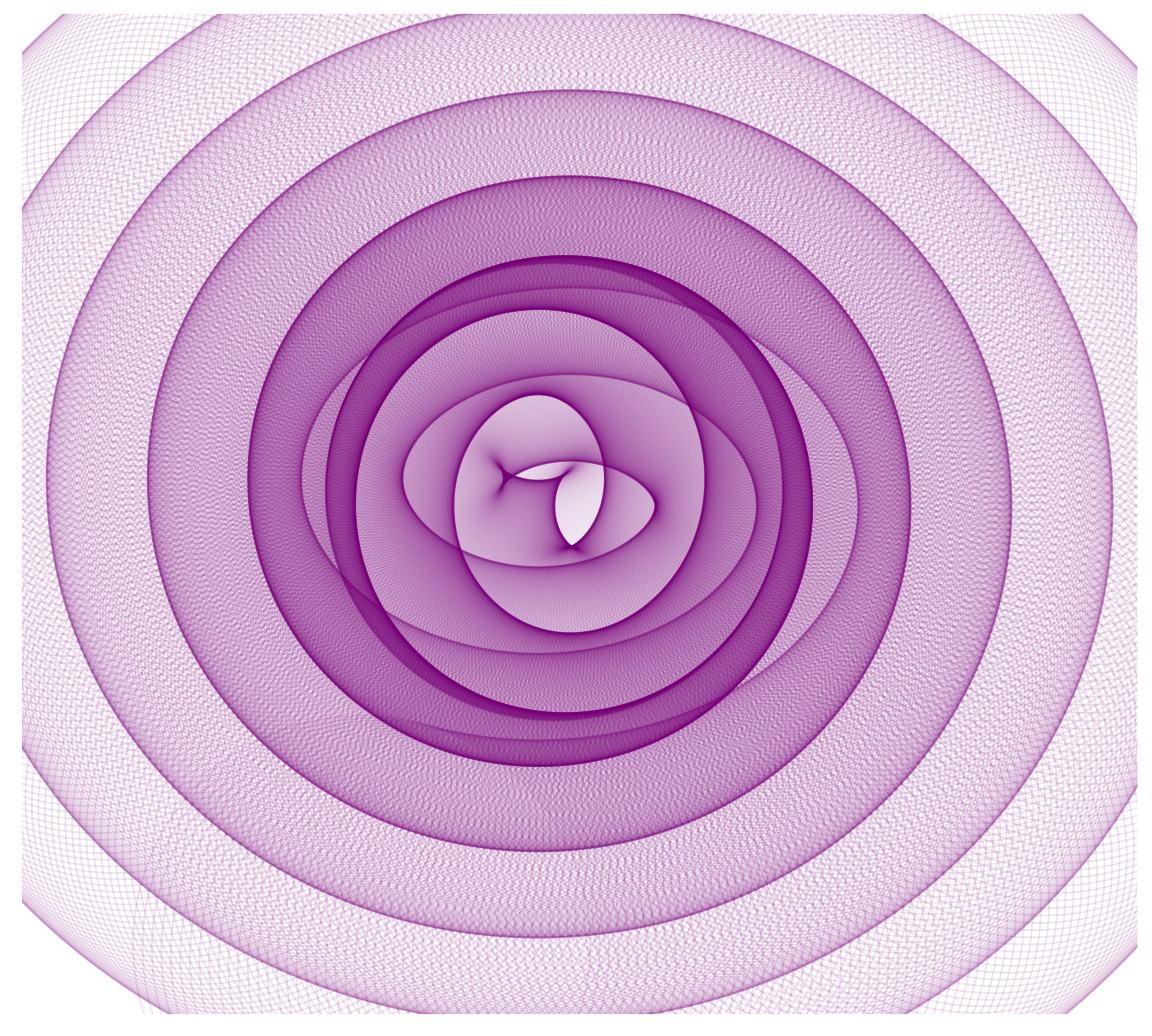
Other options
If we wanted to specify the radius we can use geom_circle which is in the ggforce package. For example, we could specify a circle with start coordinates of (3,4) and radius of 1.
library(ggforce)
# Lets make some data
circles <- tibble(x0 = 3, y0 = 4,r = 1)

# Behold the some circles
ggplot() + geom_circle(aes(x0 = x0, y0 = y0, r = r), data = circles)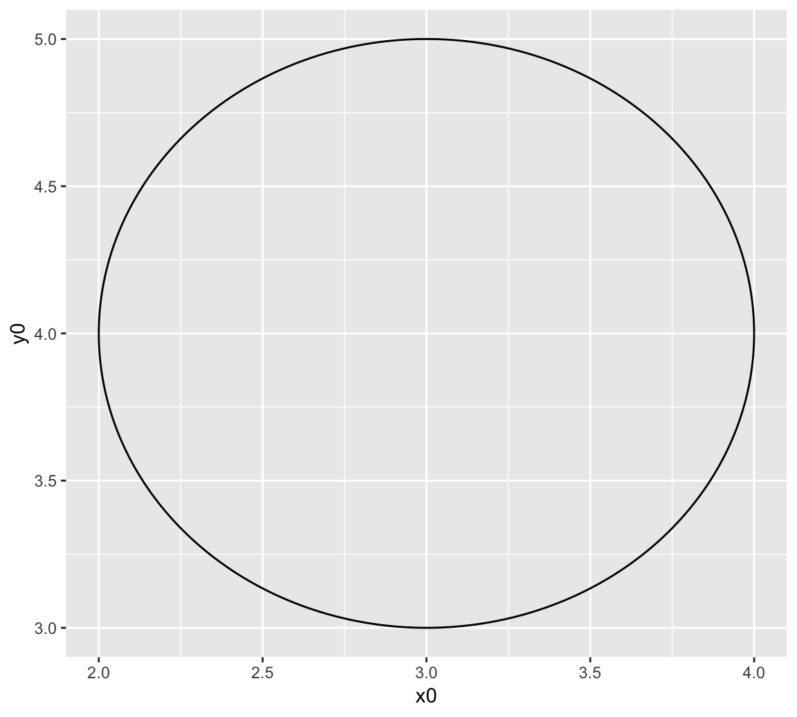
Let’s use geom_point first for the sake of comparison. Remember, the size of the circles are related to the coordinate system and not to a separate scale.
df_ggf = tibble(circle = seq(1:2500),
            x = cos((14 * pi * circle) / 2500) * (1 - (3/4)*(sin((20 * pi * circle) / 2500))^4 - (1/4)*(cos((60 * pi * circle) / 2500)) ^ 3),
            y = sin(14 * pi * circle/2500)*(1 - (3/4)*(sin(20*pi*circle/2500)) ^ 4 - (1/4)*(cos(60 * pi*circle/2500)) ^ 3),
            r = (1/120) + (1/18)*(sin(60 * pi * circle/2500))^4 + (1/18)*(sin(160*pi*circle/2500))^4)

ggplot(df_ggf, aes(x, y)) + geom_point() + theme(legend.position = "none",
        panel.grid = element_blank(),
        axis.title = element_blank(),
        axis.text = element_blank(),
        axis.ticks = element_blank(),
        panel.background = element_rect(fill = 'white'))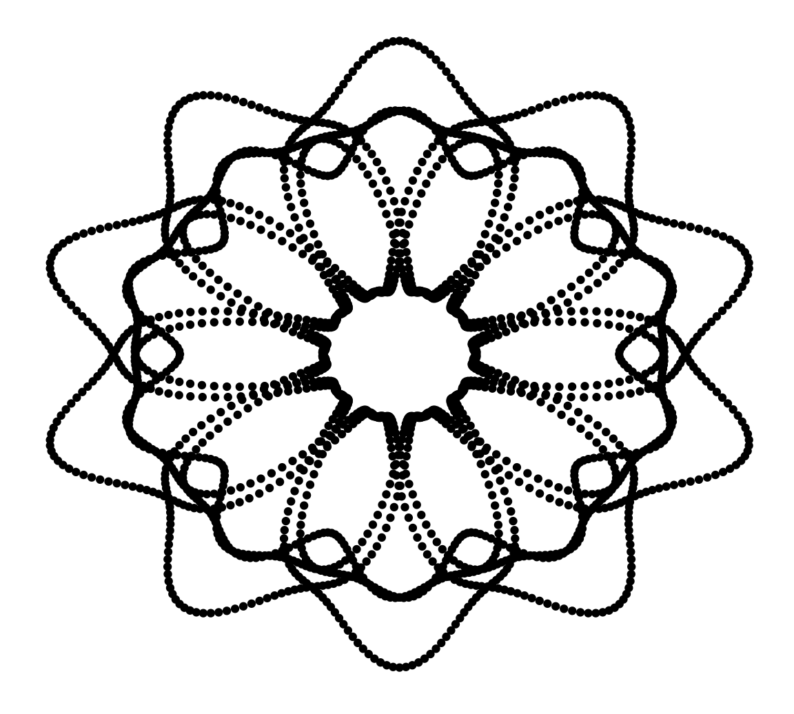
With the same dataset, let’s how to render it using geom_circle. Here, we many many different cirles put together. Every observation is a circle.
ggplot() + geom_circle(aes(x0 = x, y0 = y, r = r, fill = r), data = df_ggf) +
  theme(legend.position = "none",
        panel.grid = element_blank(),
        axis.title = element_blank(),
        axis.text = element_blank(),
        axis.ticks = element_blank(),
        panel.background = element_rect(fill = 'white')) + viridis::scale_fill_viridis()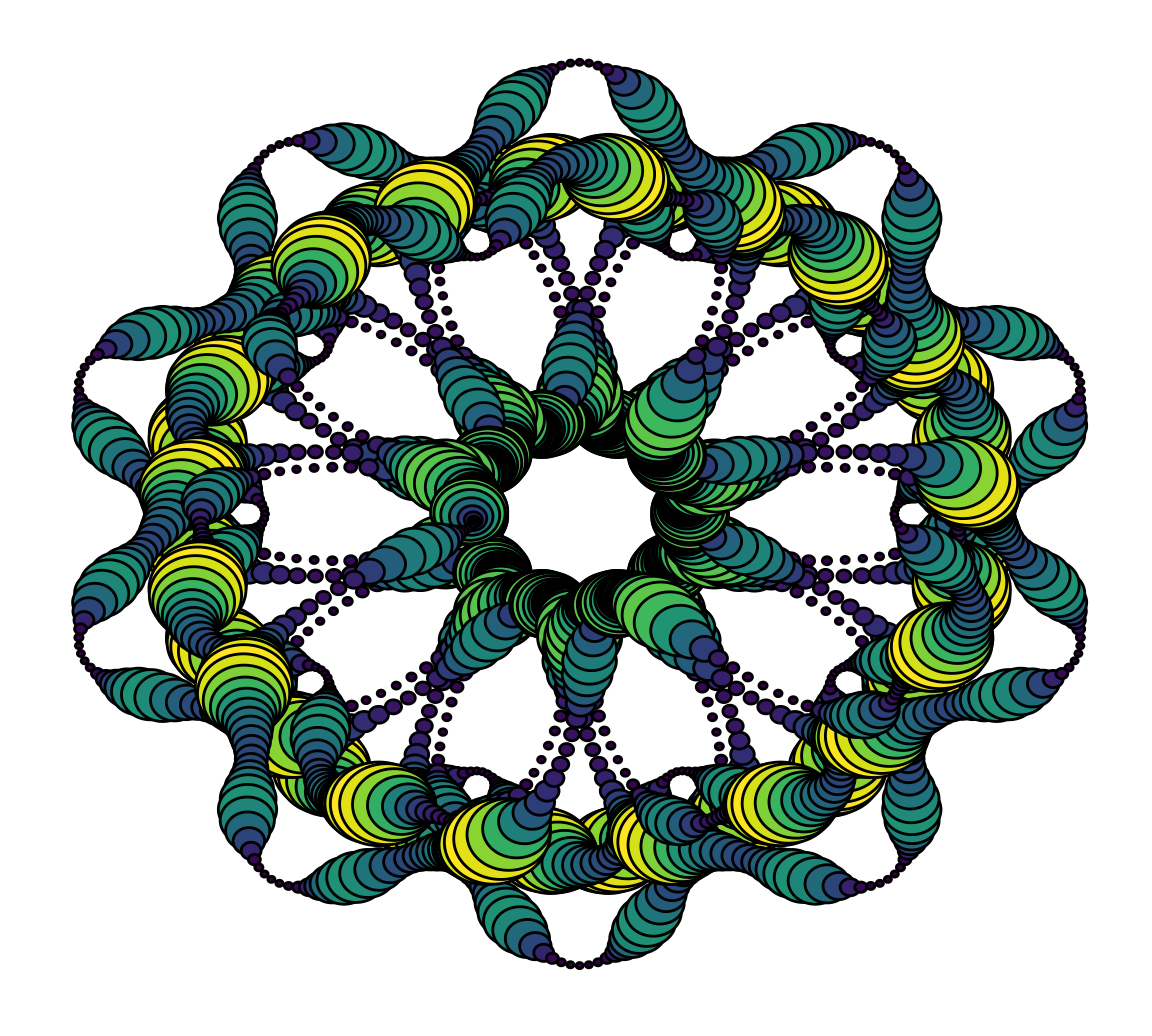
Now that was a detour. Let’s get back to our original flower. Let’s have some more fun with angles!
angle <- 12 * pi/180
points <- 2000

t <- (1:points)*angle
x <- sin(t)
y <- cos(t)

df <- data.frame(t, x, y)

p <- ggplot(df, aes(x*t, y*t))

p + geom_point(size = 80, color = 'magenta4', alpha = 0.1, shape = 1) + theme(legend.position = "none",
        panel.grid = element_blank(),
        axis.title = element_blank(),
        axis.text = element_blank(),
        axis.ticks = element_blank(),
        panel.background = element_rect(fill = 'white'))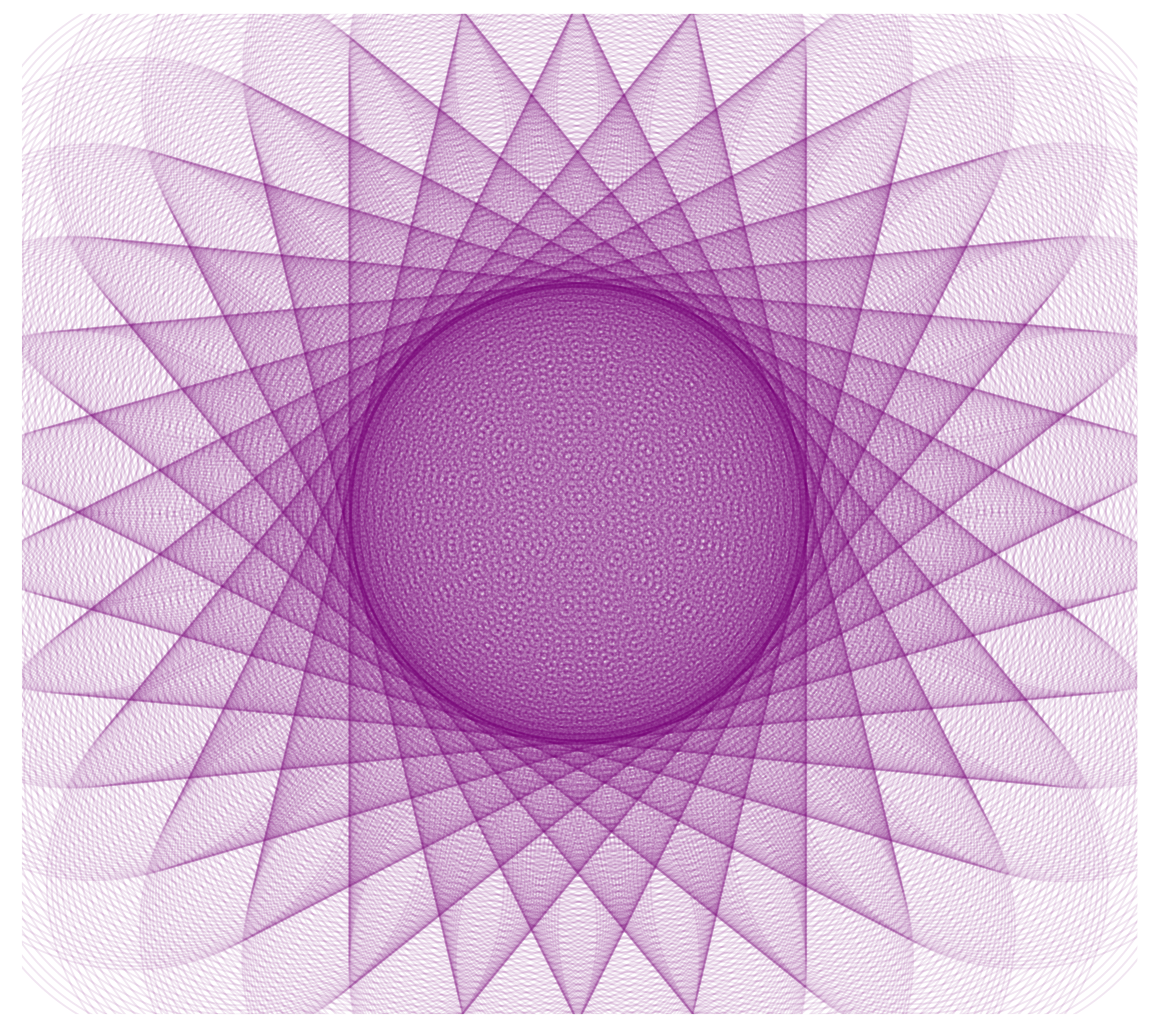
All together
Let’s set the number of points to 2000 (theoretically we can make an infinite number of patterns), change the size and color of our points.
angle <- 13 * pi/180
points <- 2000

t <- (1:points)*angle
x <- sin(t)
y <- cos(t)

df <- data.frame(t, x, y)

p <- ggplot(df, aes(x*t, y*t))

p + geom_point(size= 80, color = 'magenta4', alpha = 0.1, shape = 1) + theme(legend.position = "none",
        panel.grid = element_blank(),
        axis.title = element_blank(),
        axis.text = element_blank(),
        axis.ticks = element_blank(),
        panel.background = element_rect(fill = 'white'))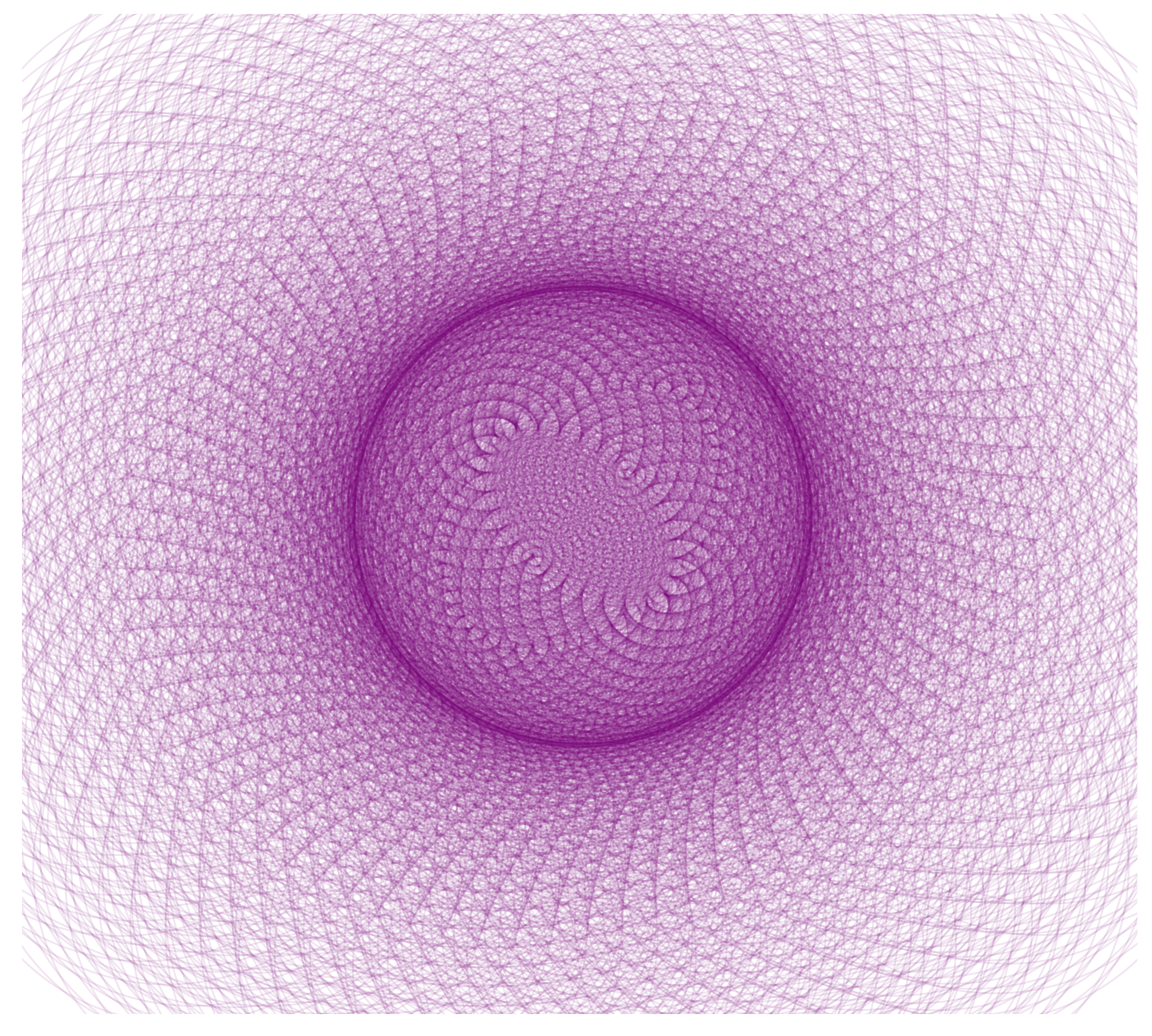
I hope you’ve enjoyed the journey between that simple circle and this beautiful flower!